After searching a lot I realized people prefer using the libraries directly for ARIMA and forecasting. To gain a better understanding,I decided to write the thing from scratch using numpy and pandas. If you feel the same way, continue reading :)

ARIMA is a model used for time-series forecasting . It has 3 main parts : Making the data stationary, AR (Auto Regression ) and MA (Moving Average). We’ll start with differencing the data ,then estimate the data using the AR ,use MA on the errors generated, un-difference the data and check the results.

I'll go over code for the model and an explanation for each step.The dataset contains the details of daily bank transactions. We’ll group the amount by month and start the analysis. Download the code and dataset here .



So many transformations exist for making the data stationary. I used log here and differencing. Subtracting the previous value didn’t make it stationary as it had a seasonal trend. Hence, I shifted the data by 12 and then subtracted it again. For example, for June 1998 we’ll subtract May 1998’s value and June 1997’s value. You can try different combinations to make sure you get the desired result. I used the ADF test to make sure the data is stationary.



For a value at time t, we assume that it is linearly dependent on the previous p lagged values and there is an error term associated with it.It is similar to linear regression, where X is the p -lagged values and y is the value at time t. Here the order p can be chosen using ACF and PACF plots, or if you have enough data just think of it as a hyper-parameter. I won’t get into the details of choosing the value of p. Here, I break the dataset into 80%–20% training and testing dataset.



The oving average part is similar to the above part. We run a linear regression on the generated residues. The code remains almost the same. Now that we have generated the coefficients and intercept, we can get our predictions. The error difference between the actual value and predicted value will form our residues.


Similar to the p, q is used here to denote the number of lagged observations. Again it can be thought of a linear regression with q-lagged errors as X and the error as y.

We now make combine the two AR and MA model to get our predictions.

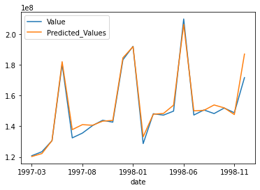
These are the final results. Looks good right?



If you have any queries or suggestions, feel free to hit me up at : dornumofficial@gmail.com. For the complete code , you can click here